Titanic Analysis
When first foraying into the world of Machine Learning (ML), there are a few very popular datasets that most students will use as a springboard to learn about the various ML algorithms on the market. The Titanic dataset is certainly one of these. The RMS Titanic was a famous ship that was designed to be ‘unsinkable’; however, as we know, it unfortunately was anything but. Upon collision with an iceberg, the Titanic sank. Of the ~2224 people on board, 68% ultimately lost their lives.
The dataset we’ll be working with contains some information about the passengers on the Titanic, and it was obtained via Kaggle. The task at hand is to, given the information in the dataset, predict whether or not a given passenger survived the sinking of the Titanic. The training data has this information, so this is an example of supervised learning. In addition, since we want to classify the passengers as either having survived or not, this is a classification problem and not a regression. Thus, we need to use a classification algorithm. I have adopted to use a Logisitic Regression, which by its name might sound like a regression but isn’t.
Below will be my analysis of the Titanic dataset as well as a training the Logistic Regression.
Import various python libraries to organize the data into a pandas DataFrame and make plots:
import pandas as pd
import numpy as np
import matplotlib.pyplot as plt
import seaborn as sns
%matplotlib inline
train = pd.read_csv('train.csv')
train.head()
| PassengerId | Survived | Pclass | Name | Sex | Age | SibSp | Parch | Ticket | Fare | Cabin | Embarked | |
|---|---|---|---|---|---|---|---|---|---|---|---|---|
| 0 | 1 | 0 | 3 | Braund, Mr. Owen Harris | male | 22.0 | 1 | 0 | A/5 21171 | 7.2500 | NaN | S |
| 1 | 2 | 1 | 1 | Cumings, Mrs. John Bradley (Florence Briggs Th... | female | 38.0 | 1 | 0 | PC 17599 | 71.2833 | C85 | C |
| 2 | 3 | 1 | 3 | Heikkinen, Miss. Laina | female | 26.0 | 0 | 0 | STON/O2. 3101282 | 7.9250 | NaN | S |
| 3 | 4 | 1 | 1 | Futrelle, Mrs. Jacques Heath (Lily May Peel) | female | 35.0 | 1 | 0 | 113803 | 53.1000 | C123 | S |
| 4 | 5 | 0 | 3 | Allen, Mr. William Henry | male | 35.0 | 0 | 0 | 373450 | 8.0500 | NaN | S |
The features in the Titanic dataset are
PassengerId: just an index that we’ll ignore except for when we submit the prediction for the test sample to Kaggle
Survived: 0 if the passenger died and 1 if they survived. Again, the fact that we have this information means we are doing supervised learning.
Pclass: The class of the passenger, either first, second, or third. For the time being, this information is being stored as an integer, but we’ll turn this into a categorical variable later on as I found that it performed better this way.
Name: The passenger name. For the time being, I will ignore this column, but it’s possible that extracting the person’s title may help.
Sex: gender by category (i.e. not represented by an integer as is the case with Pclass)
Age: self-explanitory
SibSp: Number of siblings or spouses on board
Parch: Number of parents or children on board. Note that the sum of this value and SibSp is seemingly equal to the total family size for each passenger. I decided to leave these categories alone and not just create a familySize variable because otherwise we would lose information.
Ticket: Ticket number. I just ignored this for the time being.
Fare: Price of the ticket. I left this alone other than needing to fill in a missing value, see below.
Cabin: The cabin number. Unfortunately, this is missing for the vast majority of the passengers, so I just elected to ignore it. If I were to do this analysis again, I would create a new feature that either contained the first letter of the cabin number (which is the deck of the Titanic the cabin was on) or a dummy value for the case the information was missing.
Embarked: The port from which the passenger embarked.
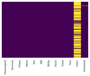
Let’s now clean the dataset from any missing values. In order to see which features have values missing, I create a heatmap to clearly show the null values:
sns.heatmap(train.isnull(),yticklabels=False,cbar=False,cmap='viridis')
<matplotlib.axes._subplots.AxesSubplot at 0x1161c6a10>
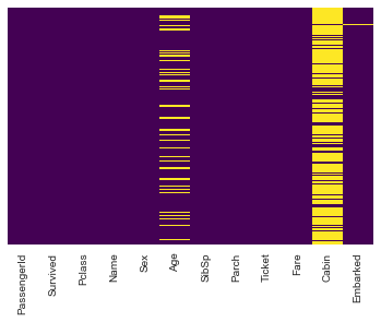
OK so it looks like we will need to deal with missing values for Age, Cabin, and Embarked. Before we do that, let’s take a look at some plots comparing some features their correlation with Survived.
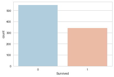
# A raw comparison of the number of survivors to the number of dead in the training set

sns.set_style('whitegrid')
sns.countplot(x='Survived',data=train,palette='RdBu_r')
<matplotlib.axes._subplots.AxesSubplot at 0x116235a10>
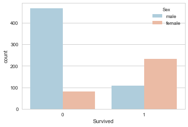
# Breakdown of survival by gender. Definitely a useful feature!

sns.set_style('whitegrid')
sns.countplot(x='Survived',hue='Sex',data=train,palette='RdBu_r')
<matplotlib.axes._subplots.AxesSubplot at 0x116334090>
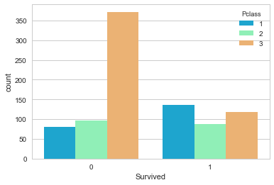
# Passenger class is also a very useful feature! The third class was much lower on the ship,
# so they were much less likely to survive.

# sns.set_style('whitegrid')
sns.countplot(x='Survived',hue='Pclass',data=train,palette='rainbow')
<matplotlib.axes._subplots.AxesSubplot at 0x1164610d0>
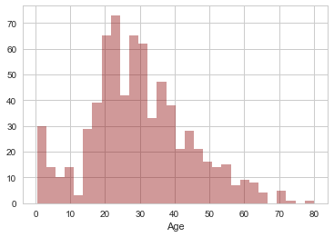
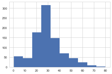
# Let's see the distribution of ages

sns.distplot(train['Age'].dropna(),kde=False,color='darkred',bins=30)
<matplotlib.axes._subplots.AxesSubplot at 0x116583a50>
OK, now let’s turn our attention to filling in the missing age values. There are a lot of passengers with missing ages, so it’s not wise to simply drop them. One simple solution would be to calculate the average age of passengers on the Titanic and just use that value for all the ones missing the age. Before we do this, let’s see if the average age differs depending on the passengers class. We’ve all seen the movie; the third class was very young while there were many older wealthy people in first class. Let’s look at a boxplot of the age distribution on the Titanic broken up by Pclass:
plt.figure(figsize=(12, 7))
sns.boxplot(x='Pclass',y='Age',data=train,palette='winter')
<matplotlib.axes._subplots.AxesSubplot at 0x1167e98d0>
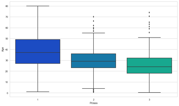
Indeed, the mean age does depend on Pclass! It would be wise to use the mean age of the passenger’s class to fill in any missing age data. Can we do one better though? What about if we use both the Pclass and the passengers gender? Let’s take a look at a boxplot of the average age broken down by both of these variables to see if further classifying by gender makes any difference:
plt.figure(figsize=(12, 7))
sns.boxplot(x='Pclass',y='Age',data=train,hue="Sex",palette='winter')
<matplotlib.axes._subplots.AxesSubplot at 0x116626890>
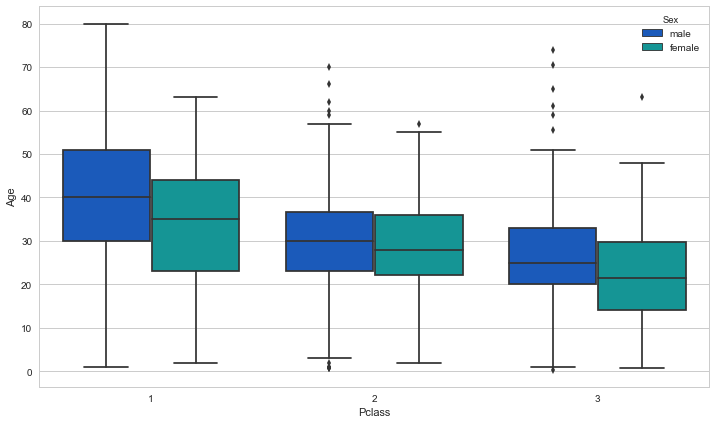
Remember, what we want to compare is not the male and female means in each Pclass, but how much do each of these differ from the average for the Pclass. The answer: not really enough to matter much. Using these means instead of just those from Pclass made no difference in the ML performance. Below I calculate the means and fill in the missing values accordingly:
# just stick with mean(Pclass) now
means = train.groupby("Pclass")["Age"].mean()
def fillAge(row):
    age = row.Age
    Pclass = row.Pclass

    if pd.isnull(age):
        return means[Pclass]
    else:
        return age

train["Age"] = train.apply(fillAge,axis=1)
The apply function above essentially loops over all the rows (i.e. passengers) in the training DataFrame, and if the age is null, then it replaces the NaN with the mean age for that passenger’s Pclass.
train["Age"].hist()
<matplotlib.axes._subplots.AxesSubplot at 0x116ab8150>
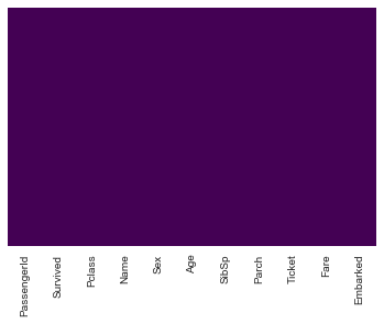
sns.heatmap(train.isnull(),yticklabels=False,cbar=False,cmap='viridis')
<matplotlib.axes._subplots.AxesSubplot at 0x1163be790>
OK, as you can see in the newly generated heatmap above, there are no more null entries for Age. Now let’s deal with Cabin and Embarked. Since so many entries are missing, I am just dropping this category altogether for the time being.
train.drop("Cabin",axis=1,inplace=True)
It looks like there’s only one passenger with the Embarked information missing. It seems safe to take the most common Embarked entry and use that:
train["Embarked"].value_counts()
S    644
C    168
Q     77
Name: Embarked, dtype: int64
# train.dropna(axis=0,inplace=True)
train["Embarked"].fillna("S",inplace=True)
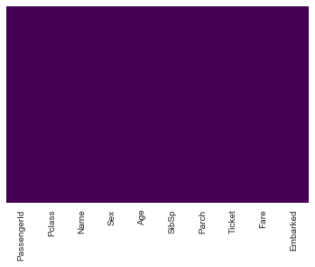
sns.heatmap(train.isnull(),yticklabels=False,cbar=False,cmap='viridis')
<matplotlib.axes._subplots.AxesSubplot at 0x116fff910>
train.head()
| PassengerId | Survived | Pclass | Name | Sex | Age | SibSp | Parch | Ticket | Fare | Embarked | |
|---|---|---|---|---|---|---|---|---|---|---|---|
| 0 | 1 | 0 | 3 | Braund, Mr. Owen Harris | male | 22.0 | 1 | 0 | A/5 21171 | 7.2500 | S |
| 1 | 2 | 1 | 1 | Cumings, Mrs. John Bradley (Florence Briggs Th... | female | 38.0 | 1 | 0 | PC 17599 | 71.2833 | C |
| 2 | 3 | 1 | 3 | Heikkinen, Miss. Laina | female | 26.0 | 0 | 0 | STON/O2. 3101282 | 7.9250 | S |
| 3 | 4 | 1 | 1 | Futrelle, Mrs. Jacques Heath (Lily May Peel) | female | 35.0 | 1 | 0 | 113803 | 53.1000 | S |
| 4 | 5 | 0 | 3 | Allen, Mr. William Henry | male | 35.0 | 0 | 0 | 373450 | 8.0500 | S |
OK we’re done filling in the missing values! Now, our last steps are to turn categorical variables into numerical ones. In pandas, this can be done very easily with pd.get_dummies().
For example,
pd.get_dummies(train.sex)
will return a pd.DataFrame with two columns, male and female, each filled with 0 or 1 depending if the passenger was male or female. Note, of course, that if male=1, female is necessarily 0 (and vice versa). Using two features that are determinalistically linked like this can lead to a problem called multicollinearity. In a case like this, we can drop one of the gender columns with no loss of information (hence the drop_first=True option below). Indeed, I do this for all categorical variables.
Note also that even though Pclass is numerical, since there are only three values, it too can be made into dummy variables.
male = pd.get_dummies(train.Sex,drop_first=True)
e = pd.get_dummies(train.Embarked,drop_first=True)
c = pd.get_dummies(train.Pclass,drop_first=True)
train = pd.concat([train,male,e,c],axis=1)
train.head()
| PassengerId | Survived | Pclass | Name | Sex | Age | SibSp | Parch | Ticket | Fare | Embarked | male | Q | S | 2 | 3 | |
|---|---|---|---|---|---|---|---|---|---|---|---|---|---|---|---|---|
| 0 | 1 | 0 | 3 | Braund, Mr. Owen Harris | male | 22.0 | 1 | 0 | A/5 21171 | 7.2500 | S | 1 | 0 | 1 | 0 | 1 |
| 1 | 2 | 1 | 1 | Cumings, Mrs. John Bradley (Florence Briggs Th... | female | 38.0 | 1 | 0 | PC 17599 | 71.2833 | C | 0 | 0 | 0 | 0 | 0 |
| 2 | 3 | 1 | 3 | Heikkinen, Miss. Laina | female | 26.0 | 0 | 0 | STON/O2. 3101282 | 7.9250 | S | 0 | 0 | 1 | 0 | 1 |
| 3 | 4 | 1 | 1 | Futrelle, Mrs. Jacques Heath (Lily May Peel) | female | 35.0 | 1 | 0 | 113803 | 53.1000 | S | 0 | 0 | 1 | 0 | 0 |
| 4 | 5 | 0 | 3 | Allen, Mr. William Henry | male | 35.0 | 0 | 0 | 373450 | 8.0500 | S | 1 | 0 | 1 | 0 | 1 |
# drop all original columns we used to make the dummy coluns and also name and ticket which we won't use

train.drop("Sex",axis=1,inplace=True)
train.drop("Pclass",axis=1,inplace=True)
train.drop("Embarked",axis=1,inplace=True)
train.drop("Name",axis=1,inplace=True)
train.drop("Ticket",axis=1,inplace=True)
train.head()
| PassengerId | Survived | Age | SibSp | Parch | Fare | male | Q | S | 2 | 3 | |
|---|---|---|---|---|---|---|---|---|---|---|---|
| 0 | 1 | 0 | 22.0 | 1 | 0 | 7.2500 | 1 | 0 | 1 | 0 | 1 |
| 1 | 2 | 1 | 38.0 | 1 | 0 | 71.2833 | 0 | 0 | 0 | 0 | 0 |
| 2 | 3 | 1 | 26.0 | 0 | 0 | 7.9250 | 0 | 0 | 1 | 0 | 1 |
| 3 | 4 | 1 | 35.0 | 1 | 0 | 53.1000 | 0 | 0 | 1 | 0 | 0 |
| 4 | 5 | 0 | 35.0 | 0 | 0 | 8.0500 | 1 | 0 | 1 | 0 | 1 |
OK, let’s do all these steps with the test sample. Note that since this is from Kaggle, the test sample doesn’t come with the value for Survived; this is for us to determine via using Logistic Regression on the training sample!
test = pd.read_csv("test.csv")
# sns.heatmap(test.isnull(),yticklabels=False,cbar=False,cmap='viridis')
test.drop("Cabin",axis=1,inplace=True)
test["Age"] = test.apply(fillAge,axis=1)
test["Embarked"].fillna("S",inplace=True)
test["Fare"].fillna(test[test.Fare.notnull()]["Fare"].mean(),inplace=True)
# test.dropna(axis=0,inplace=True)
# test.Fare.isnull().value_counts()
sns.heatmap(test.isnull(),yticklabels=False,cbar=False,cmap='viridis')
<matplotlib.axes._subplots.AxesSubplot at 0x1170f1e90>
male = pd.get_dummies(test.Sex,drop_first=True)
e = pd.get_dummies(test.Embarked,drop_first=True)
c = pd.get_dummies(test.Pclass,drop_first=True)
test = pd.concat([test,male,e,c],axis=1)
test.drop("Sex",axis=1,inplace=True)
test.drop("Pclass",axis=1,inplace=True)
test.drop("Embarked",axis=1,inplace=True)
test.drop("Name",axis=1,inplace=True)
test.drop("Ticket",axis=1,inplace=True)
test.head()
| PassengerId | Age | SibSp | Parch | Fare | male | Q | S | 2 | 3 | |
|---|---|---|---|---|---|---|---|---|---|---|
| 0 | 892 | 34.5 | 0 | 0 | 7.8292 | 1 | 1 | 0 | 0 | 1 |
| 1 | 893 | 47.0 | 1 | 0 | 7.0000 | 0 | 0 | 1 | 0 | 1 |
| 2 | 894 | 62.0 | 0 | 0 | 9.6875 | 1 | 1 | 0 | 1 | 0 |
| 3 | 895 | 27.0 | 0 | 0 | 8.6625 | 1 | 0 | 1 | 0 | 1 |
| 4 | 896 | 22.0 | 1 | 1 | 12.2875 | 0 | 0 | 1 | 0 | 1 |
Now, what I will do is to split the training set further into a training and testing set and then train the model on this smaller training set. Later on, we will train on the entire training set using a grid search and cross-validation.
from sklearn.model_selection import train_test_split
X_train,X_test,y_train,y_test = train_test_split(train.drop("PassengerId",axis=1).drop("Survived",axis=1),train["Survived"], test_size=0.3, random_state=101)
from sklearn.linear_model import LogisticRegression
logmodel = LogisticRegression()
logmodel.fit(X_train,y_train)
LogisticRegression(C=1.0, class_weight=None, dual=False, fit_intercept=True,
          intercept_scaling=1, max_iter=100, multi_class='ovr', n_jobs=1,
          penalty='l2', random_state=None, solver='liblinear', tol=0.0001,
          verbose=0, warm_start=False)
predictions = logmodel.predict(X_test)
from sklearn.metrics import classification_report,confusion_matrix

print confusion_matrix(y_test,predictions)
print classification_report(y_test,predictions)
[[138  16]
 [ 40  74]]
             precision    recall  f1-score   support

          0       0.78      0.90      0.83       154
          1       0.82      0.65      0.73       114

avg / total       0.80      0.79      0.79       268
test.head()
| PassengerId | Age | SibSp | Parch | Fare | male | Q | S | 2 | 3 | |
|---|---|---|---|---|---|---|---|---|---|---|
| 0 | 892 | 34.5 | 0 | 0 | 7.8292 | 1 | 1 | 0 | 0 | 1 |
| 1 | 893 | 47.0 | 1 | 0 | 7.0000 | 0 | 0 | 1 | 0 | 1 |
| 2 | 894 | 62.0 | 0 | 0 | 9.6875 | 1 | 1 | 0 | 1 | 0 |
| 3 | 895 | 27.0 | 0 | 0 | 8.6625 | 1 | 0 | 1 | 0 | 1 |
| 4 | 896 | 22.0 | 1 | 1 | 12.2875 | 0 | 0 | 1 | 0 | 1 |
predictions = logmodel.predict(test.drop("PassengerId",axis=1))
test.info()
test["Survived"]=predictions
test.shape
<class 'pandas.core.frame.DataFrame'>
RangeIndex: 418 entries, 0 to 417
Data columns (total 10 columns):
PassengerId    418 non-null int64
Age            418 non-null float64
SibSp          418 non-null int64
Parch          418 non-null int64
Fare           418 non-null float64
male           418 non-null uint8
Q              418 non-null uint8
S              418 non-null uint8
2              418 non-null uint8
3              418 non-null uint8
dtypes: float64(2), int64(3), uint8(5)
memory usage: 18.4 KB


(418, 11)
test[["PassengerId","Survived"]].to_csv("logreg_pclassdummy.csv",index=False)
test.drop("Survived",axis=1,inplace=True) # drop so we can re-evaluate
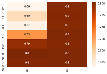
The above analysis was done without any tuning of the model parameters. Also, we trained the model on just one subset of the training sample! Of course, the exact model efficiency is dependent on the split used in the training, but hopefully this is a small effect. Also, we’d like to train using the entire training sample! We will find the parameters that gave the best performance under cross-validation and then retrain using the entire training dataset with those parameters with GridSearchCV. Let’s see how much difference this makes:
gridVals = {'penalty': ['l1','l2'], 'C': [0.001,0.01,0.1,1,10,100,1000]}
from sklearn.model_selection import GridSearchCV

X = train.drop("PassengerId",axis=1).drop("Survived",axis=1)
y = train["Survived"]

grid_search = GridSearchCV(LogisticRegression(), gridVals, cv=5)
grid_search.fit(X,y)
print "Best parameters: {}".format(grid_search.best_params_)
print "Best cross-validation score: {:.2f}".format(grid_search.best_score_)
Best parameters: {'penalty': 'l2', 'C': 0.1}
Best cross-validation score: 0.80
results = pd.DataFrame(grid_search.cv_results_)
scores = np.array(results.mean_test_score).reshape(2, 7)
scores = pd.DataFrame(scores).T
scores.columns = gridVals["penalty"]
scores.index = gridVals["C"]
sns.heatmap(scores,cmap="Oranges",annot=True)
<matplotlib.axes._subplots.AxesSubplot at 0x117bbc6d0>
predictions = grid_search.predict(test.drop("PassengerId",axis=1))
test["Survived"]=predictions
test[["PassengerId","Survived"]].to_csv("logreg_pclassdummy_gridsearchcv.csv",index=False)