Allstate Insurance Claim Value
The following is my solution to a Kaggle contest that ran in early 2017 regarding predicting the value of insurance claim payout as a function of many different given features. For privacy purposes (and also to protect internal information I assume), all of the variables are anonymized. There are a mix of both continuous and categorical variables, with the latter providing the vast majority of the features in the dataset. In order to treat the categorical variables, we must ‘one-hot-encode’ them, so for each combination of categorical variable and possible value for that variable, we create a new column with either a 0 if the entry doesn’t have this characteristic or 1 if it does.
import numpy as np
import matplotlib.pyplot as plt
import pandas as pd
import seaborn as sns

plt.rcParams["patch.force_edgecolor"] = True
%matplotlib inline
train = pd.read_csv("train.csv")
train.head()
| id | cat1 | cat2 | cat3 | cat4 | cat5 | cat6 | cat7 | cat8 | cat9 | ... | cont6 | cont7 | cont8 | cont9 | cont10 | cont11 | cont12 | cont13 | cont14 | loss | |
|---|---|---|---|---|---|---|---|---|---|---|---|---|---|---|---|---|---|---|---|---|---|
| 0 | 1 | A | B | A | B | A | A | A | A | B | ... | 0.718367 | 0.335060 | 0.30260 | 0.67135 | 0.83510 | 0.569745 | 0.594646 | 0.822493 | 0.714843 | 2213.18 |
| 1 | 2 | A | B | A | A | A | A | A | A | B | ... | 0.438917 | 0.436585 | 0.60087 | 0.35127 | 0.43919 | 0.338312 | 0.366307 | 0.611431 | 0.304496 | 1283.60 |
| 2 | 5 | A | B | A | A | B | A | A | A | B | ... | 0.289648 | 0.315545 | 0.27320 | 0.26076 | 0.32446 | 0.381398 | 0.373424 | 0.195709 | 0.774425 | 3005.09 |
| 3 | 10 | B | B | A | B | A | A | A | A | B | ... | 0.440945 | 0.391128 | 0.31796 | 0.32128 | 0.44467 | 0.327915 | 0.321570 | 0.605077 | 0.602642 | 939.85 |
| 4 | 11 | A | B | A | B | A | A | A | A | B | ... | 0.178193 | 0.247408 | 0.24564 | 0.22089 | 0.21230 | 0.204687 | 0.202213 | 0.246011 | 0.432606 | 2763.85 |
5 rows × 132 columns
Let’s first check if there’s any missing values in the dataset:
train.isnull().sum().sum()
0
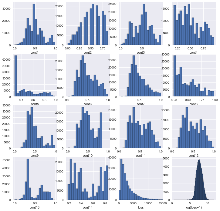
Let’s now take a look at the distributions for the continuous variables. Note that I’ve added a plot that transforms the claim loss to log(loss+1). The reason for this is that the log function fixes the skewness of the loss distribution, and this will make the regression perform better. I choose log(loss+1) instead of just log(loss) to cover the case if loss = 0 and to assure the transformed variable is positive (recall that the log of a number between 0 and 1 is negative). If some of the target variable space is negative, this will also throw off the regression. It’s possible that some of the other continuous features would benefit from this treatment as well, but I’ll leave that to another time. Of course, once the prediction is made, the inverse function exp(x)-1 will transform the variable back to dollars (presumably this is the unit, we are never told).
plt.subplots(4,4,figsize=(12,12))
for i in range(1,15):
    plt.subplot(4,4,i)
    plt.hist(train["cont%i"%i],bins=20)
    plt.xlabel("cont%i"%i)

plt.subplot(4,4,15)
plt.hist(train["loss"],bins=200)
plt.xlim(0,15000)
plt.xlabel("loss")

plt.subplot(4,4,16)
plt.hist(np.log1p(train["loss"]),bins=200)
# plt.xlim(0,15000)
plt.xlabel("log(loss+1)")
<matplotlib.text.Text at 0x114570ad0>
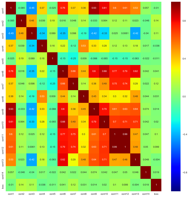
Now let’s check out the correlation matrix for all the continuous variables:
contVars = ["cont"+"%i"%i for i in range(1,15)]
contVars.append("loss")
plt.figure(figsize=(14,14))
sns.heatmap(train[contVars].corr(),annot=True,cmap="jet")
<matplotlib.axes._subplots.AxesSubplot at 0x111f03750>
Now, let’s do the one-hot-encoding of the training and test samples. I temporarily merge the training and test samples in order to do this because what can (and does in this case) happen is that the test sample will have options for some categorical variables that the training does not have, so the columns in each case would be different.
train["isTest"]=False

test = pd.read_csv("test.csv")
test["isTest"] = True
test["loss"] = np.pi
a = pd.concat([train,test])
a = pd.get_dummies(a,drop_first=True)
train = a[a.isTest==False].copy()
test = a[a.isTest==True].copy()
train.drop("isTest",axis=1,inplace=True)
test.drop("isTest",axis=1,inplace=True)
del a
test.drop("loss",axis=1,inplace=True)
Split up the training sample into a training and test sample in order to train and test the regression. Remember that the test sample we defined in the cell above was the one given by Kaggle without the target variable, so we can’t use it to test our model. Also recall that I transform the loss to log(loss + 1) in order to correct the skewness of the distribution.
from sklearn.model_selection import train_test_split

X = train.drop("loss",axis=1).drop("id",axis=1)
y = np.log1p(train["loss"])

X_train, X_test, y_train, y_test = train_test_split(X, y, test_size=0.3, random_state=42)
I use a Linear Support Vector Regressor (LinearSVR) to model the dependence of the loss upon the features given in the dataset. Remember that, of course, after making a prediction with the regression, we must invert the transformation with exp(y) - 1. The MAE I get is competitive in the Kaggle competition, which is nice for such a quick exercise!
from sklearn.svm import LinearSVR
from sklearn.metrics import *

clf = LinearSVR()
clf.fit(X_train,y_train)
pred = clf.predict(X_test)

y_testTrans = np.expm1(y_test)
predTrans = np.expm1(pred)

print mean_absolute_error(y_testTrans,predTrans)
print mean_squared_error(y_testTrans,predTrans)
print np.sqrt(mean_squared_error(y_testTrans,predTrans))

testX = test.drop("id",axis=1)
testPred = np.expm1(clf.predict(testX))
test["loss"] = testPred
test[["id","loss"]].to_csv("linearSVR.csv",index=False)
test.drop("loss",axis=1,inplace=True)
1269.39779994
7593361.65182
2755.6054964
For my last step, I’ll perform cross-validation of the model across the training sample to see how well the model generalizes. Since the scores are all similar in value, we’re doing well on this front.
from sklearn.model_selection import cross_val_score
scores = cross_val_score(clf, X_train, y_train, cv=5)
print scores
[ 0.50818537 0.50933825 0.52031112 0.51211244 0.51128369]